Small demo of the needed elements to load, analyze and print a time series in Python. Format of the data-source:
...
2019-08-28,11701.019531,EUR
2019-08-29,11838.879883,EUR
2019-08-30,11939.280273,EUR
2019-09-02,11953.780273,EUR
2019-09-03,11910.860352,EUR
2019-09-04,12025.040039,EUR
2019-09-05,12126.780273,EUR
2019-09-06,12191.730469,EUR
2019-09-09,12226.099609,EUR
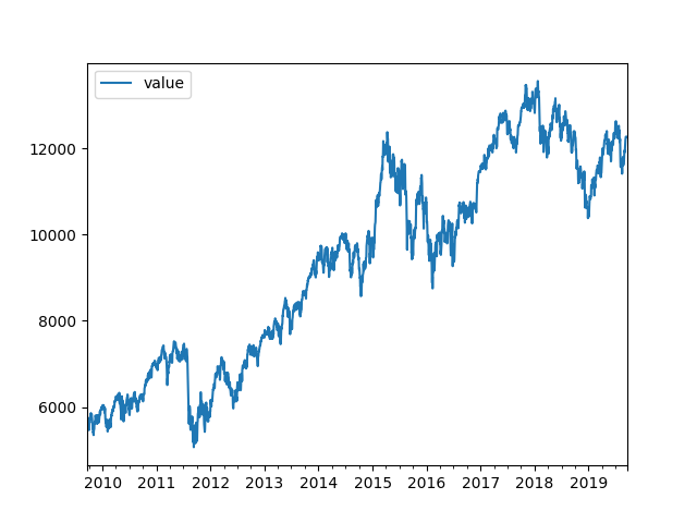
2019-09-10,12268.709961,EURGenerates based on the complete data, the annual average performance and volatility
Annual Performance:  8.026639312445006
Annual Vola:  19.100050116208784
… and the plot of the analyzed data:
… based on the following code:
#!/usr/bin/python3

import numpy as np
import pandas as pd
import matplotlib.pyplot as plt
from datetime import datetime, date

# some variables
now = datetime.now() # date/time of software execution
endDate = date(year = now.year, month = now.month, day = now.day) # date of software execution (end of analytics period)
startDate = date(year = now.year-10, month = now.month, day = now.day) # 1 year earlies (begin of analytics period)
deltaYears = (endDate-startDate).days/365.2425 # difference of startDate and endDate in years

# read csv file & build timeseries
# raw = pd.read_csv("./Reference/stocks_2/JP3942600002.EUR.csv", header=None)
raw = pd.read_csv("./DAX.EUR.csv", header=None)

ts = pd.DataFrame(columns=['datetime','value']) # generate timeframe
ts['datetime'] = pd.to_datetime(raw[0]) # load column-datetime with the raw-timestamps
ts['value'] = raw[1] # load column-value with the values
ts = ts.set_index('datetime') # index based on datetime
# print(ts)

# reduction of timeseries to the choosen period and cleaning for weekdays
ts = ts.resample('D').ffill() # generate sample size one-day and fill missing elements
selection = pd.date_range(startDate, endDate, freq='B') # generat selection from startDate to endDate with weekdays
ts = ts.asof(selection) # get subset of ts according selection and interpolate remaining ()
# print(ts)

# some calculation
val = np.array(ts['value'])
res = np.log(val[1:]/val[:(len(val)-1)])
# r = (np.power(1+np.mean(res),len(res))-1)*100 # performance
r = (np.power(np.power(1+np.mean(res),len(res)),1/deltaYears)-1)*100 # performance (annual)
v = np.std(res)*np.sqrt(len(res))*100/np.sqrt(deltaYears) # vola (annual)
print('Annual Performance: ',r)
print('Annual Vola: ',v)

# check
ts.head()

# plot
ts.plot()
plt.show()