Loose or tight coupling experience

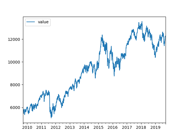
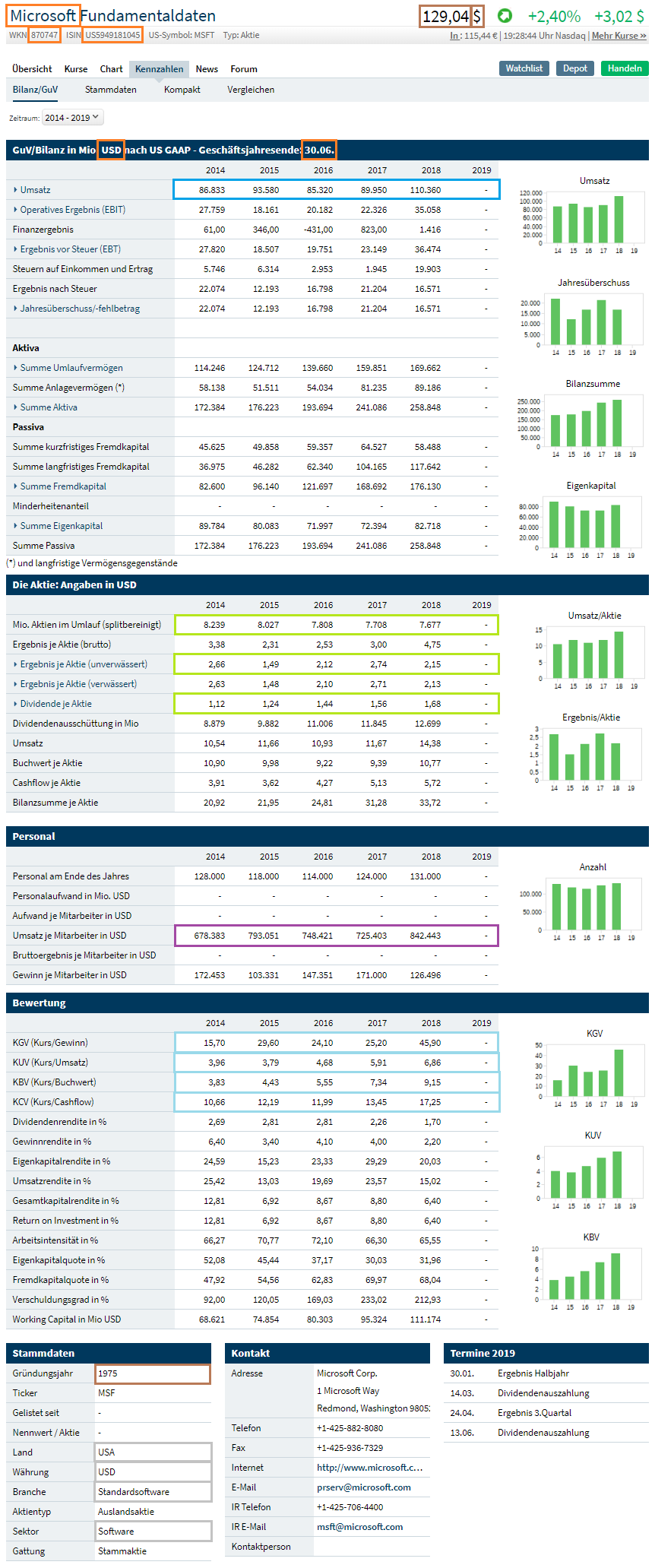
The target is to get some time series data in any currency, multiply it with an FX and store it in EUR. First approach was something like:

  1. “crawl time series and write in table a”.py everyhour
  2. “crawl fx time series and write in table b”.py everyhour
  3. “read table a & read table b, multiply and write in table c”.py everyhour

Everything went well and I came up with the idea: “Could the third step not be done by the MySQL-db itself?”

  1. “crawl time series and write in table a”.py everyhour
  2. “crawl fx time series and write in table b”.py everyhour
  3. table a uses the AFTER INSERT & AFTER UPDATE function to trigger the transformation and storage in table c. As example added the following code to table a:

CREATE DEFINER=wolfgang@localhost TRIGGER raw_cps_AFTER_INSERT AFTER INSERT ON raw_cps FOR EACH ROW BEGIN
IF NEW.currency = 'USD' THEN
SELECT USD FROM investment_db.ts_pivot_currency WHERE date=NEW.date INTO @FX;
SET @value_fx = NEW.value/@FX;
INSERT INTO investment_db.fun_cps (pk, date, value,currency)
VALUES(NEW.pk, NEW.date, @value_fx, 'EUR')
ON DUPLICATE KEY UPDATE value=@value_fx, currency='EUR';
END IF;
END

… and then i noticed that i get an error in my “crawl time series and write in table a”.py. There was data in table a. Conclusion step (1) = ok. Also there was a lot of data in table b and table c. So was step (2) and step (3) = ok. No!

Tight coupling introduced by mistake!

Because of one missing FX entry, the multiplication failed and due to that the error was transferred to the python script. Because the script was running in an container and some quick and dirty programming, it was permanently restarted 😉

Analyzing Timeseries with Python

Small demo of the needed elements to load, analyze and print a time series in Python. Format of the data-source:

...
2019-08-28,11701.019531,EUR
2019-08-29,11838.879883,EUR
2019-08-30,11939.280273,EUR
2019-09-02,11953.780273,EUR
2019-09-03,11910.860352,EUR
2019-09-04,12025.040039,EUR
2019-09-05,12126.780273,EUR
2019-09-06,12191.730469,EUR
2019-09-09,12226.099609,EUR
2019-09-10,12268.709961,EUR

Generates based on the complete data, the annual average performance and volatility

Annual Performance:  8.026639312445006
Annual Vola:  19.100050116208784

… and the plot of the analyzed data:

… based on the following code:

#!/usr/bin/python3 

import numpy as np
import pandas as pd
import matplotlib.pyplot as plt
from datetime import datetime, date

# some variables
now = datetime.now() # date/time of software execution
endDate = date(year = now.year, month = now.month, day = now.day) # date of software execution (end of analytics period)
startDate = date(year = now.year-10, month = now.month, day = now.day) # 1 year earlies (begin of analytics period)
deltaYears = (endDate-startDate).days/365.2425 # difference of startDate and endDate in years

# read csv file & build timeseries
# raw = pd.read_csv("./Reference/stocks_2/JP3942600002.EUR.csv", header=None)
raw = pd.read_csv("./DAX.EUR.csv", header=None)

ts = pd.DataFrame(columns=['datetime','value']) # generate timeframe
ts['datetime'] = pd.to_datetime(raw[0]) # load column-datetime with the raw-timestamps
ts['value'] = raw[1] # load column-value with the values
ts = ts.set_index('datetime') # index based on datetime
# print(ts)

# reduction of timeseries to the choosen period and cleaning for weekdays
ts = ts.resample('D').ffill() # generate sample size one-day and fill missing elements
selection = pd.date_range(startDate, endDate, freq='B') # generat selection from startDate to endDate with weekdays
ts = ts.asof(selection) # get subset of ts according selection and interpolate remaining ()
# print(ts)

# some calculation
val = np.array(ts['value'])
res = np.log(val[1:]/val[:(len(val)-1)])
# r = (np.power(1+np.mean(res),len(res))-1)*100 # performance
r = (np.power(np.power(1+np.mean(res),len(res)),1/deltaYears)-1)*100 # performance (annual)
v = np.std(res)*np.sqrt(len(res))*100/np.sqrt(deltaYears) # vola (annual)
print('Annual Performance: ',r)
print('Annual Vola: ',v)

# check
ts.head()

# plot 
ts.plot()
plt.show()

Find Potential Investments II

The Target View

At the end I want a table to find fast the items that might be interesting to be more investigated. This is structured in the following way:

variablecomment
isinISIN Code is used as the guiding element.
Also all the data files will be named according that identifier.
nameName of the company to be aware what to reed
dateDate of the last crawl to detect a broken pipeline, too

Find Potential Investments

The Purpose

There is an uncountable number of potential investments and chances existing in the world. Why not get them searched and reduced to a data set that might be investigated more deep to find the “right” one?

Solution is a very tailored crawler written in Python.

The Data Model

Crawling a page it is possible to extract some relevant data.